Run cell-based matching

This takes as set of input metadetect catalogs and runs matching using the cell-based ShearMatch matcher.

Standard imports

[1]:

import hpmcm
import glob
import os
import numpy as np
import matplotlib.pyplot as plt

Set up the configuration

[2]:

DATADIR = "test_data"   # Input data directory
shear_st = "0p01"       # Applied shear as a string
shear = 0.01            # Decimal version of applied shear
shear_type = "wmom"     # which object characterization to use
tract = 10463           # which tract to study

SOURCE_TABLEFILES = sorted(glob.glob(os.path.join(DATADIR, f"shear_{shear_type}_{shear_st}_uncleaned_{tract}_*.pq")))
SOURCE_TABLEFILES.reverse()
VISIT_IDS = np.arange(len(SOURCE_TABLEFILES))

PIXEL_R2CUT = 4.         # Cut at distance**2 = 4 pixels
PIXEL_MATCH_SCALE = 1    # Use pixel scale to do matching

Make the matcher, reduce the data

[3]:

matcher = hpmcm.ShearMatch.createShearMatch(pixelR2Cut=PIXEL_R2CUT, pixelMatchScale=PIXEL_MATCH_SCALE, deshear=-1*shear)

[4]:

matcher.reduceData(SOURCE_TABLEFILES, VISIT_IDS)

This should have made 200 x 200 cells

[5]:

matcher.n_cell

[5]:

array([200., 200.])

Run the data

Note the option to run all the cells. By default we only run a small subset for testing

[6]:

do_partial = True
if do_partial:
    x_range = range(50, 70)
    y_range = range(170, 190)
    #xRange = [55]
    #yRange = [170]
    matcher.analysisLoop(x_range, y_range)
else:
    matcher.analysisLoop()

 50!
......... 60!
......... Done!

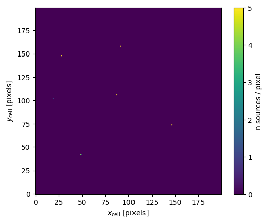
Show the source counts map for a single cell

The x and y axes here are the in the cell frame. The color scale shows the number of sources per/pixel. The analysis looks for clusters of adjacent pixels with counts.

[7]:

cell = matcher.cell_dict[matcher.getCellIdx(50, 170)]
od = cell.analyze(None, 4)
_ = plt.imshow(od['counts_map'], origin='lower')
_ = plt.colorbar(label="n sources / pixel")
_ = plt.xlabel(r"$x_{\rm cell}$ [pixels]")
_ = plt.ylabel(r"$y_{\rm cell}$ [pixels]")

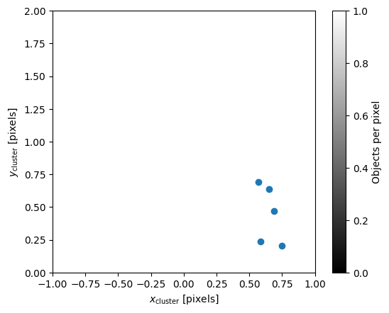
Show a single cluster

The x and y axes here are the in the cluster frame for a single cluster. The color scale shows the number of sources per/pixel.

The x markers are the original source postions. The o makters are the deshear positions.

[8]:

cluster = list(cell.cluster_dict.values())[0]
fig = hpmcm.viz_utils.showCluster(od['image'], cluster, cell)
_ = fig.axes[0].set_xlim(-1, 1)
_ = fig.axes[0].set_ylim(0, 2)
_ = fig.axes[0].set_xlabel(r"$x_{\rm cluster}$ [pixels]")
_ = fig.axes[0].set_ylabel(r"$y_{\rm cluster}$ [pixels]")

Extract the output of the matching

There are a few empty cells to play around with the output data.

stats and shear_stats are both tuples of pandas.DataFrame

[9]:

stats = matcher.extractStats()
shear_stats = matcher.extractShearStats()
obj_shear = shear_stats[1]

[10]:

stats[0]

[10]:

	cluster_id	source_id	source_idx	catalog_id	distance	cell_idx
0	10170004	165811	0	0	0.008754	10170
1	10170004	165615	0	1	0.052315	10170
2	10170004	165601	0	2	0.051875	10170
3	10170004	165706	1	3	0.044073	10170
4	10170004	165350	0	4	0.038651	10170
...	...	...	...	...	...	...
33	13989002	203175	7	0	0.002944	13989
34	13989002	202967	7	1	0.031898	13989
35	13989002	202882	6	2	0.029662	13989
36	13989002	203019	7	3	0.018704	13989
37	13989002	202591	6	4	0.017916	13989

12932 rows × 6 columns

Get the offsets between the cluster centroid and the sources

This is to check that the deshearing is correctly applied

[11]:

def get_offsets(matcher):
    n = 0
    dd = {
        0:dict(dx=[], dy=[], x=[], y=[]),
        1:dict(dx=[], dy=[], x=[], y=[]),
        2:dict(dx=[], dy=[], x=[], y=[]),
        3:dict(dx=[], dy=[], x=[], y=[]),
        4:dict(dx=[], dy=[], x=[], y=[]),
    }
    for cellData in matcher.cell_dict.values():
        n += len(cellData.data[0])
        for obj in cellData.object_dict.values():
            if not obj.n_unique == 5 and obj.n_src == 5:
                continue
            for iCat in range(5):
                mask = obj.catalog_id == iCat
                if mask.sum() == 0:
                    continue
                for dx, dy in zip((obj.x_pix[mask] - obj.x_cent), (obj.y_pix[mask] - obj.y_cent)):
                    dd[iCat]["dx"].append(dx)
                    dd[iCat]["dy"].append(dy)
                    dd[iCat]["x"].append(float(obj.data[mask].iloc[0].x_cell))
                    dd[iCat]["y"].append(float(obj.data[mask].iloc[0].y_cell))

    for i in range(5):
        dd[i]['dx'] = np.array(dd[i]['dx'])
        dd[i]['dy'] = np.array(dd[i]['dy'])
        dd[i]['x'] = np.array(dd[i]['x'])
        dd[i]['y'] = np.array(dd[i]['y'])
    print(n)
    return dd

[12]:

dd = get_offsets(matcher)

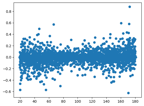
Plots the residuals, they should be flat

[13]:

_ = plt.scatter(dd[4]['x'], dd[4]['dx'])

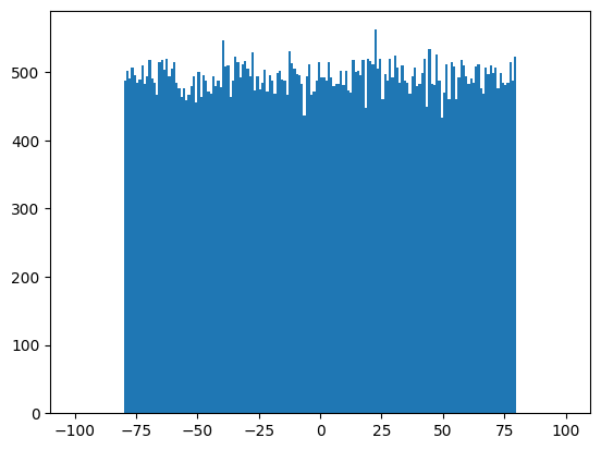
Look at how the sources lie within the cells

[14]:

_ = plt.hist(matcher.full_data[0].x_cell_coadd, bins=np.linspace(-100, 100, 201))

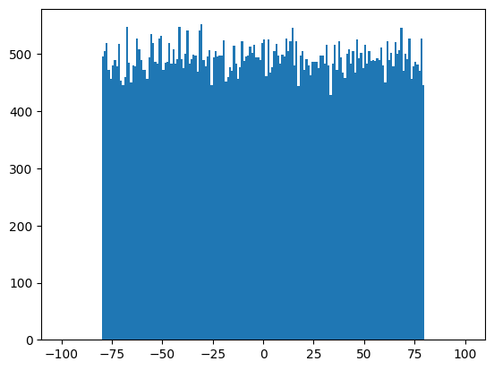
[15]:

_ = plt.hist(matcher.full_data[0].y_cell_coadd, bins=np.linspace(-100, 100, 201))

Classify the objects by match type

This looks at the characteristics of the matched objects and categorizes them.

[16]:

obj_lists = hpmcm.classify.classifyObjects(matcher, snr_cut=10.)
hpmcm.classify.printObjectTypes(obj_lists)

All Objects:                                    2767
cut 1                                           374
cut 2                                           38
Used:                                           2355
good (n source from n catalogs):                1031
good faint                                      1133
faint (< n sources, snr < cut):                 181
mixed (n source from < n catalogs):             0
edge_mixed (mixed near edge of cell):           0
edge_missing (< n sources, near edge of cell):  0
edge_extra (> n sources, near edge of cell):    0
faint (< n sources, snr < cut):                 181
orphan (split off from larger cluster           7
one missing (n-1 sources, not near edge):       0
two missing (n-2 sources, not near edge):       0
many missing (< n-2 sources, not near edge):    3
extra (> n sources, not near edge):             0

Measure the matching efficiency for objects above the SNRCut

[17]:

n_good = len(obj_lists['ideal'])
bad_list = ['edge_mixed', 'edge_missing', 'edge_extra', 'orphan', 'missing', 'two_missing', 'many_missing', 'extra', 'caught']
n_bad = np.sum([len(obj_lists[x]) for x in bad_list])
effic = n_good/(n_good+n_bad)
effic_err = np.sqrt(effic*(1-effic)/(n_good+n_bad))
print(f"Effic: {effic:.5} +- {effic_err:.5f}")

Effic: 0.99039 +- 0.00302

Classify the clusters by match type

This looks at the characteristics of the matched cluster and categorizes them.

[18]:

cluster_lists = hpmcm.classify.classifyClusters(matcher, snr_cut=10.)
hpmcm.classify.printClusterTypes(cluster_lists)

All Clusters:                                   2745
cut 1                                           372
cut 2                                           38
Used:                                           2335
good (n source from n catalogs):                1031
good faint                                      1135
faint (< n sources, snr < cut):                 165
mixed (n source from < n catalogs):             0
edge_mixed (mixed near edge of cell):           0
edge_missing (< n sources, near edge of cell):  0
edge_extra (> n sources, near edge of cell):    0
faint (< n sources, snr < cut):                 165
one missing (n-1 sources, not near edge):       0
two missing (n-2 sources, not near edge):       0
many missing (< n-2 sources, not near edge):    3
extra (> n sources, not near edge):             1

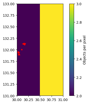
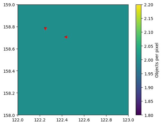
Display a few objects

The various markers show the sources from different shear catalogs: ns=., 1m = <, 1p = >, 2m = ^, 2p = v.

[19]:

_ = hpmcm.viz_utils.showShearObjs(matcher, cluster_lists['ideal'][5])

[20]:

_ = hpmcm.viz_utils.showShearObj(matcher, obj_lists['many_missing'][0])

[ ]:

[ ]:

[ ]: