Extract the efficiency of the matching between the shear catalogs

Since they all use the same source detection, the only differences should come from differences in the applied noise

Standard imports

import tables_io
import numpy as np
import hpmcm
import matplotlib.pyplot as plt

Set up the configuration

keys = ['_cluster_stats', '_cluster_shear']  # which tables to read
st_ = 'wmom'          # which catalog type
shear_st_ = "0p01"    # Applied shear as a string
tract = 10463         # which tract to study

dd = tables_io.read(f"test_data/shear_{st_}_{shear_st_}_match_{tract}.pq", keys=keys)
data = dd['_cluster_stats']
data2 = dd['_cluster_shear']

column_list None
column_list None

Merge the two tables we read

data["idx"] = np.arange(len(data))
data2["idx"] = np.arange(len(data2))
merged = data.merge(data2, on="idx")
merged['has_ref_cat'] = merged.n_ns > 0
merged['central'] = np.bitwise_and(
    np.fabs(merged.x_cent-100) < 75,
    np.fabs(merged.y_cent-100) < 75,
)
central = merged[merged.central]

Make maskes of different types of matches

good_mask = np.bitwise_and(central.n_src ==5, central.n_unique ==5)
missing_md = np.bitwise_and(~good_mask, central.has_ref_cat)
missing_ref = np.bitwise_and(~good_mask, ~central.has_ref_cat)
extra = central.n_src > central.n_unique

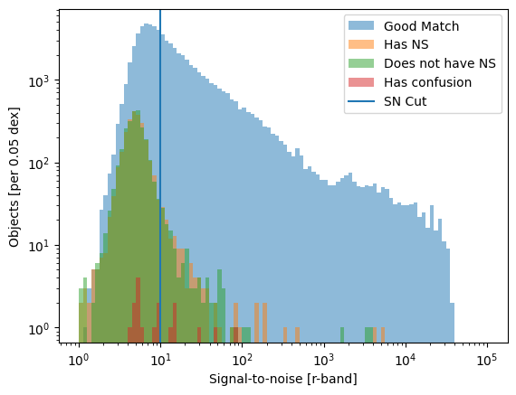
Make a histogram of the different match types

_ = plt.hist(central.iloc[good_mask.values].snr, bins=np.logspace(0, 5, 101), alpha=0.5, label="Good Match")
_ = plt.hist(central.iloc[missing_md.values].snr, bins=np.logspace(0, 5, 101), alpha=0.5, label="Has NS")
_ = plt.hist(central.iloc[missing_ref.values].snr, bins=np.logspace(0, 5, 101), alpha=0.5, label="Does not have NS")
_ = plt.hist(central.iloc[extra.values].snr, bins=np.logspace(0, 5, 101), alpha=0.5, label="Has confusion")
_ = plt.axvline(10, label='SN Cut')
_ = plt.xscale('log')
_ = plt.yscale('log')
_ = plt.legend()
_ = plt.xlabel("Signal-to-noise [r-band]")
_ = plt.ylabel("Objects [per 0.05 dex]")

hist_all =  np.histogram(central.snr, bins=np.logspace(0, 5, 101))[0]
hist_missing_md = np.histogram(central.iloc[missing_md.values].snr, bins=np.logspace(0, 5, 101))[0]
hist_missing_ref = np.histogram(central.iloc[missing_ref.values].snr, bins=np.logspace(0, 5, 101))[0]
hist_extra = np.histogram(central.iloc[extra.values].snr, bins=np.logspace(0, 5, 101))[0]

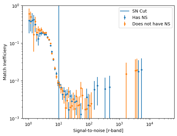
Estimate the good match efficiency as a function of SNR

ineffic_missing_md = hist_missing_md/hist_all
ineffic_missing_ref = hist_missing_ref/hist_all
ineffic_extra = hist_extra/hist_all
npq_missing_md = np.sqrt(ineffic_missing_md*(1-ineffic_missing_md)/hist_all)
npq_missing_ref = np.sqrt(ineffic_missing_ref*(1-ineffic_missing_ref)/hist_all)
npq_missing_extra = np.sqrt(ineffic_extra*(1-ineffic_extra)/hist_all)
bin_edges = np.logspace(0, 5, 101)
bin_centers = np.sqrt(bin_edges[0:-1] * bin_edges[1:])

/tmp/ipykernel_1543/3171407875.py:1: RuntimeWarning: invalid value encountered in divide
  ineffic_missing_md = hist_missing_md/hist_all
/tmp/ipykernel_1543/3171407875.py:2: RuntimeWarning: invalid value encountered in divide
  ineffic_missing_ref = hist_missing_ref/hist_all
/tmp/ipykernel_1543/3171407875.py:3: RuntimeWarning: invalid value encountered in divide
  ineffic_extra = hist_extra/hist_all

Plot the good match efficiency as a function of SNR

_ = plt.errorbar(bin_centers, ineffic_missing_md, yerr=npq_missing_md, label="Has NS", ls="", marker='.')
_ = plt.errorbar(bin_centers, ineffic_missing_ref, yerr=npq_missing_ref, label="Does not have NS", ls="", marker='.')
_ = plt.xscale('log')
_ = plt.yscale('log')
_ = plt.ylim(1e-3,1)
_ = plt.axvline(10, label='SN Cut')
_ = plt.xlabel("Signal-to-noise [r-band]")
_ = plt.ylabel("Match Inefficieny")
_ = plt.legend()